PLDS State Estimation Tutorial #

This tutorial shows how to use this library to estimate the state of an LDS with Poisson observations from input/output data. In place of a physical system, another PLDS model (lds::poisson::System) receives random inputs and provides measurements for the state estimator. For the sake of example, the only parameter mismatch is assumed to be the process disturbance, which is adaptively re-estimated.

The full code for this can be found here.

Preamble #

In addition to including the main ldsCtrlEst header, this tutorial will use some shorthand.

#include <ldsCtrlEst>

using lds::Matrix;
using lds::Vector;
using lds::data_t;
using std::cout;

Note that lds::Matrix and lds::Vector are typedefs for arma::Mat<data_t> and arma::Col<data_t>, where the data type is double by default. May be changed to float in include/ldsCtrlEst_h/lds.h if there are memory constraints (e.g., large-scale MIMO control problems).

Creating a simulated system #

A first-order single-input/single-output system will be used for the purposes of this demonstration. The simulation will be run at 1 kHz for 30 seconds.

  // Make SISO system sampled at 1kHz
  data_t dt = 1e-3;
  size_t n_u = 1;                           // no. inputs
  size_t n_x = 1;                           // no. states
  size_t n_y = 1;                           // no. outputs
  auto n_t = static_cast<size_t>(30 / dt);  // no time steps for simulation.

When a system is initialized, rather than requiring all parameters be provided at construction, users may create a default system by setting only the dimensions and sample period.

  // construct ground truth system...
  lds::poisson::System system_true(n_u, n_x, n_y, dt);

This default system is a random walk, where the state matrix is identity, the input matrix is zeros, and the top min(n_x, n_y) states are observed at the output. i.e., for this example, \[ x_{t+1} = x_t + w_t \]

where \( w_{t} \sim \mathcal{N}\left( 0, Q \right) \) .

Now, create non-default parameters for this model.

  // Model parameters
  Matrix a_true(n_x, n_x, arma::fill::eye);
  a_true[0] = exp(-dt / 0.075);
  Matrix b_true = Matrix(n_x, n_u).fill(1e-2);
  Vector m0_true = Vector(n_x, arma::fill::zeros).fill(-7e-2);  // disturbance
  Vector x0_true = m0_true * arma::inv(Matrix(n_x, n_x, arma::fill::eye) -
                                        a_true);  // initial state

Finally, assign the parameters using corresponding set-methods.

  // Assign params.
  system_true.set_A(a_true);
  system_true.set_B(b_true);
  system_true.set_x0(x0_true);
  system_true.set_m(m0_true);
  system_true.Reset();

Creating the estimator #

Now, create the estimator. The system type includes filtering functionality for state estimation, so create another lds::poisson::System. As noted above, the only parameter mismatch in this simulation will be the process disturbance.

  // Construct system for estimation
  // e.g., will create a model with incorrect disturbance
  lds::poisson::System system_estimator(n_u, n_x, n_y, dt);

  // Can copy parameters from another system object
  system_estimator = system_true;

  // wrong disturbance
  Vector m0_est = m0_true * 2;
  system_estimator.set_m(m0_est);

  // set new initial conditions
  Vector x0_est = m0_est * arma::inv(Matrix(n_x, n_x, arma::fill::eye) -
                                      a_true);  // initial state
  system_estimator.set_x0(x0_est);
  system_estimator.Reset();  // reset to initial condition.

To ensure robust estimates, adaptively re-estimate the process disturbance.

  // turn on adaptive disturbance estimation
  system_estimator.do_adapt_m = true;

  // set adaptation rate by changing covariance of assumed process noise acting
  // on random-walk evolution of m
  Matrix q_m = Matrix(n_x, n_x, arma::fill::eye) * 1e-6;
  system_estimator.set_Q_m(q_m);

Simulating estimation #

In this demonstration, random inputs are presented to the system, measurements are taken, and filtering is carried out in a for-loop.

    // Simlate the true system.
    z.col(t) = system_true.Simulate(u.col(t - 1));

    // Filter (predict -> update)
    system_estimator.Filter(u.col(t - 1), z.col(t));

Example simulation result #

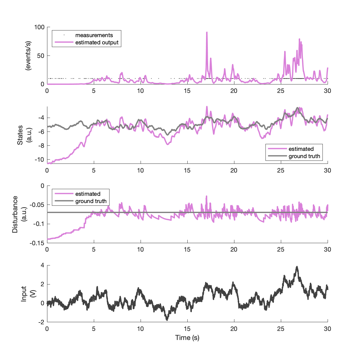
Below are example results for this simulation, including outputs, latent states, process disturbance, and the input. The online estimates of the output, state, and disturbance are given in purple.

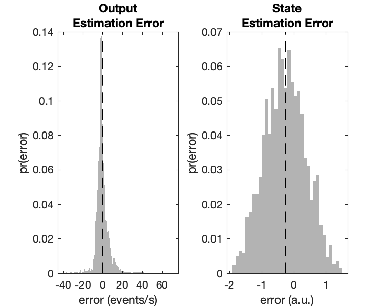
With this parameterization, it takes the estimator approximately 5 seconds to minimize state error. The state and output error distributions for the period after 5 seconds is shown below.