GLDS Control Tutorial #

This tutorial shows how to use this library to control a system with a Gaussian LDS controller (lds::gaussian::Controller). In place of a physical system, a GLDS model (lds::gaussian::System) receives control inputs and simulates measurements for the feedback control loop. The controller is assumed to have an imperfect model of the system being controlled (here, a gain mismatch), and there is a stochastic, unmeasured disturbance acting on the system. A combination of integral action and adaptive estimation of this process disturbance is used to perform control.

The full code for this can be found here.

Preamble #

In addition to including the main ldsCtrlEst header, this tutorial will use some shorthand.

#include <ldsCtrlEst>

using lds::Matrix;
using lds::Vector;
using lds::data_t;
using std::cout;

Note that lds::Matrix and lds::Vector are typedefs for arma::Mat<data_t> and arma::Col<data_t>, where the data type is double by default. May be changed to float in include/ldsCtrlEst_h/lds.h if there are memory constraints (e.g., large-scale MIMO control problems).

Creating a simulated system #

A first-order single-input/single-output system will be used for the purposes of this demonstration. The simulation will be run at 1 kHz for 5 seconds.

  // Make 1st-order SISO system, sampled at 1kHz
  data_t dt = 1e-3;
  size_t n_u = 1;
  size_t n_x = 1;
  size_t n_y = 1;

  // no time steps for simulation.
  auto n_t = static_cast<size_t>(5.0 / dt);

When a system is initialized, rather than requiring all parameters be provided at construction, users may create a default system by setting only the dimensions and sample period.

  // construct ground truth system to be controlled...
  // initializes to random walk model with top-most n_y state observed
  lds::gaussian::System controlled_system(n_u, n_x, n_y, dt);

This default system is a random walk, where the state matrix is identity, the input matrix is zeros, and the top min(n_x, n_y) states are observed at the output. i.e., for this example, \[ x_{t+1} = x_t + w_t \]

\[ y_{t} = x_t \]

where \( w_{t} \sim \mathcal{N}\left( 0, Q \right) \) .

Now, create non-default parameters for this model.

  // Ground-truth parameters for the controlled system
  // (stand-in for physical system to be controlled)
  Matrix a_true(n_x, n_x, arma::fill::eye);
  a_true[0] = exp(-dt / 0.01);
  Matrix b_true = Matrix(n_x, n_u).fill(2e-4);
  // control signal to model input unit conversion e.g., V -> mW/mm2:
  Vector g_true = Vector(n_y).fill(10.0);

  // output noise covariance
  Matrix r_true = Matrix(n_y, n_y, arma::fill::eye) * 1e-4;

As mentioned above, this example will feature a stochastic disturbance. More specifically, a process disturbance will randomly change between two values.

  /// Going to simulate a switching disturbance (m) acting on system
  size_t which_m = 0;  // whether low or high disturbance (0, 1)
  data_t m_low = 5 * dt * (1 - a_true[0]);
  data_t pr_lo2hi = 1e-3;  // probability of going from low to high disturb.
  data_t m_high = 20 * dt * (1 - a_true[0]);
  data_t pr_hi2lo = pr_lo2hi;

  // initially let m be low
  Vector m0_true = Vector(n_y).fill(m_low);

Finally, assign the parameters using corresponding set-methods.

 // Assign params.
  controlled_system.set_A(a_true);
  controlled_system.set_B(b_true);
  controlled_system.set_m(m0_true);
  controlled_system.set_g(g_true);
  controlled_system.set_R(r_true);

Creating the controller #

Now, create the controller. This requires first constructing the system model that the control uses for estimating state feedback and updating the control signal. A controller is then constructed from this lds::gaussian::System object and upper/lower bounds on the control signal (u_lb, u_ub below), past which the control saturates. Here, the control signal is command voltage sent to an analog driver (e.g., for an LED). Its limits are 0 to 5 V. If your actuator does not saturate somehow, simply set the lower and upper bounds to -lds::kInf and lds::kInf, respectively. Simple saturation is currently the only actuator model in this library.

For the sake of this simulation, the system model input matrix is set to an incorrect value. We also assume that the controller feedback gains were designed with an actuator whose conversion factor from volts to physical units (e.g., mW/mm2 optical intensity) differed from the actuator being used in the current experiment.

  // make a controller
  lds::gaussian::Controller controller;
  {
    // Create **incorrect** model used for control.
    // (e.g., imperfect model fitting)
    Matrix b_controller = b_true / 2;

    // let's assume zero process disturbance initially
    // (will be re-estimating)
    Vector m_controller = Vector(n_x, arma::fill::zeros);

    // for this demo, just use arbitrary default R
    Matrix r_controller = Matrix(n_y, n_y, arma::fill::eye) * lds::kDefaultR0;

    lds::gaussian::System controller_system(controlled_system);
    controller_system.set_B(b_controller);
    controller_system.set_m(m_controller);
    controller_system.set_R(r_controller);
    controller_system.Reset();  // reset to new m

    // going to adaptively re-estimate the disturbance
    controller_system.do_adapt_m = true;

    // set adaptation rate by changing covariance of assumed process noise
    // acting on random-walk evolution of m
    Matrix q_m = Matrix(n_x, n_x, arma::fill::eye) * 1e-6;
    controller_system.set_Q_m(q_m);

    // create controller
    // lower and upper bounds on control signal (e.g., in Volts)
    data_t u_lb = 0.0;  // [=] V
    data_t u_ub = 5.0;  // [=] V
    controller = std::move(
        lds::gaussian::Controller(std::move(controller_system), u_lb, u_ub));
  }

Note that the above code block demonstrates how move semantics can be used for assignment/construction. Copy assignment/construction is of course also allowed.

With the controller constructed, control variables may be set.

  // Control variables:
  // if following enabled, adapts set point with re-estimated process
  // disturbance n.b., should not need integral action if this is enabled as the
  // adaptive estimator minimizes DC error
  bool do_adaptive_set_point = false;

  // Reference/target output, controller gains
  Vector y_ref0 = Vector(n_y).fill(20.0 * dt);
  Matrix k_x = Matrix(n_u, n_x).fill(100);     // gains on state error
  Matrix k_inty = Matrix(n_u, n_y).fill(1e3);  // gains on integrated err

  // setting initial state to target to avoid error at onset:
  Vector x0 = Vector(n_x).fill(y_ref0[0]);

  // set up controller type bit mask so controller knows how to proceed
  size_t control_type = 0;
  if (do_adaptive_set_point) {
    // adapt set point with estimated disturbance
    control_type = control_type | lds::kControlTypeAdaptM;
  } else {
    // use integral action to minimize DC error
    control_type = control_type | lds::kControlTypeIntY;
  }

  // set controller type
  controller.set_control_type(control_type);

  // Let's say these controller gains were designed assuming g was 9 V/(mW/mm2):
  Vector g_design = Vector(n_u).fill(9);

  // Set params.
  // **n.b. using arbitrary defaults for Q, R in this example. Really, these
  // should be set by users, as they tune characteristics of Kalman filter.
  // Users can also choose not to recursively calculate the estimator gain and
  // supply it (setKe) instead of covariances.**
  controller.set_y_ref(y_ref0);
  controller.set_Kc(k_x);
  controller.set_Kc_inty(k_inty);
  controller.set_g_design(g_design);

Simulating control #

In this demonstration, we will use the ControlOutputReference method which allows users to simply set the reference output and supply the current measurement z. It then calculates the solution for the state/input required to track the reference output at steady state. In this case, the goal is to regulate the output about a constant reference, so it is appropriate here. This method can also be used for time-varying references as long as this variation is slow compared to the dynamics of the system.

The control loop is carried out here in a simple for-loop, where a the controlled system is simulated, a measurement taken, and the control signal updated.

  // Simulate the true system.
  z.col(t) = controlled_system.Simulate(u_tm1);

  // This method uses a steady-state solution to control problem to calculate
  // x_ref, u_ref from reference output y_ref. Therefore, it is only
  // applicable to regulation problems or cases where reference trajectory
  // changes slowly compared to system dynamics.
  u.col(t) = controller.ControlOutputReference(z.col(t));

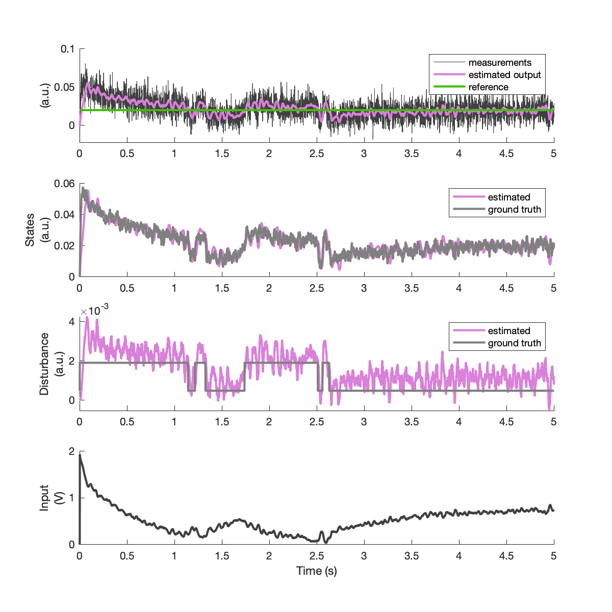
Example simulation result #

Below are example results for this simulation, including outputs, latent states, process disturbance, and the control signal. The controller’s online estimates of the output, state, and disturbance are given in purple.

example control output